A YOLO Segmentation Model for Grocery Items!
Summary
An experiment to train a model to detect Filipino grocery items using YOLO. YOLO v11 model (X-size) is trained in this experiment for object detection and segmentation tasks for common Filipino grocery items under a variety of model configurations and data augmentation techniques. An inference application is deployed via tunneling on a Gradio interface.
Prompt
The idea was simple — create a product detection or segmentation model using the most common Filipino grocery items, with as many of them as possible. We did this as a class for the UPD MEngAI AI 231 course, Machine Learning Operations (here’s a helpful link to Dr. Rowel Atienza’s GitHub repository for the Deep Learning course). Obviously, the first step was building a database of images, and doing manual annotation. It wasn’t the easiest experience, but it definitely made us appreciate a lot of the struggle.
Having a model that could do this was a simple proof of concept — we didn’t have to go too far and fine-tune Optical Character Recognition (OCR) and Open-Vocabulary Object Detection (OVOD) models. I decided to do supervised training with the Ultralytics YOLO - v11 series. At this time, the Segment Anything Models were already released, but YOLO models were simply smaller, faster, and more computationally efficient. See the table below for a quick comparison from the Ultralytics website.
| Model | Size (Mb) | Parameters (M) | Speed (CPU) (ms/im) |
|---|---|---|---|
| Meta SAM-b | 375 | 93.7 | 49401 |
| MobileSAM | 40.7 | 10.1 | 25381 |
| FastSAM-s with YOLOv8 backbone | 23.7 | 11.8 | 55.9 |
| Ultralytics YOLOv8n-seg | 6.7 (11.7x smaller) | 3.4 (11.4 less) | 24.5 (1061x faster) |
| Ultralytics YOLO11n-seg | 5.9 (13.2x smaller) | 2.9 (13.4 less) | 30.1 (864x faster) |
The idea was to find a model that was robust enough to detect even at varying conditions. It was easier said than done.
Methodology and Rationale of Proposed Solution
Part 1
This was composed of Run 1 to 14 configurations. Our class had 2 weeks to come up with initial solutions, aside from doing the data collection, preprocessing, and annotation. Each had to present an individual solution and deliberate the pros and cons of the solution. We also had to present a demo and share our findings with the entire class.
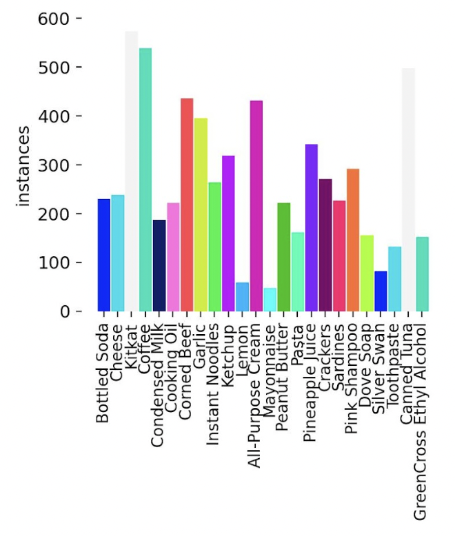
There was no known dataset yet on Filipino grocery products so our class had to split the data collection duties. I had focused on collecting pictures of UFC Banana Ketchup. The full dataset contained about 500 images per object class. Take a look at the items the other people had to collect in the table below.
| Common Grocery Item | Specific Details |
|---|---|
| Bottled Soda | Coke Zero |
| Canned Sardines | 555 Sardines |
| Canned Tuna | Century Tuna (short and tall cans, white label) |
| Cheese | Eden Cheese (box and sachet) |
| Chocolate | KitKat |
| Coffee | Nescafé 3-in-1 Original (single & twin pack) |
| Condensed Milk | Alaska Classic (377 g can) |
| Cooking Oil | Simply Pure Canola Oil |
| Corned Beef | Purefoods Corned Beef |
| Crackers | Rebisco Crackers (transparent packaging) |
| Ethyl Alcohol | Green Cross |
| Garlic | Whole bulb of garlic |
| Instant Noodles | Lucky Me Pancit Canton |
| Ketchup | UFC Banana Ketchup |
| Lemon | Whole lemon |
| Mayonnaise | Lady’s Choice Real Mayonnaise (220 ml jar) |
| Nestlé All-Purpose Cream | Nestlé – 250 ml |
| Pasta | Spaghetti or macaroni |
| Peanut Butter | Skippy |
| Pineapple Juice | Del Monte Green (Fiber and ACE variants) |
| Shampoo | Pink Sunsilk |
| Soap | Dove Relaxing Lavender |
| Soy Sauce | Silver Swan Soy Sauce (385 ml) |
| Toothpaste | Colgate Advanced White Value Pack (2 tubes) |
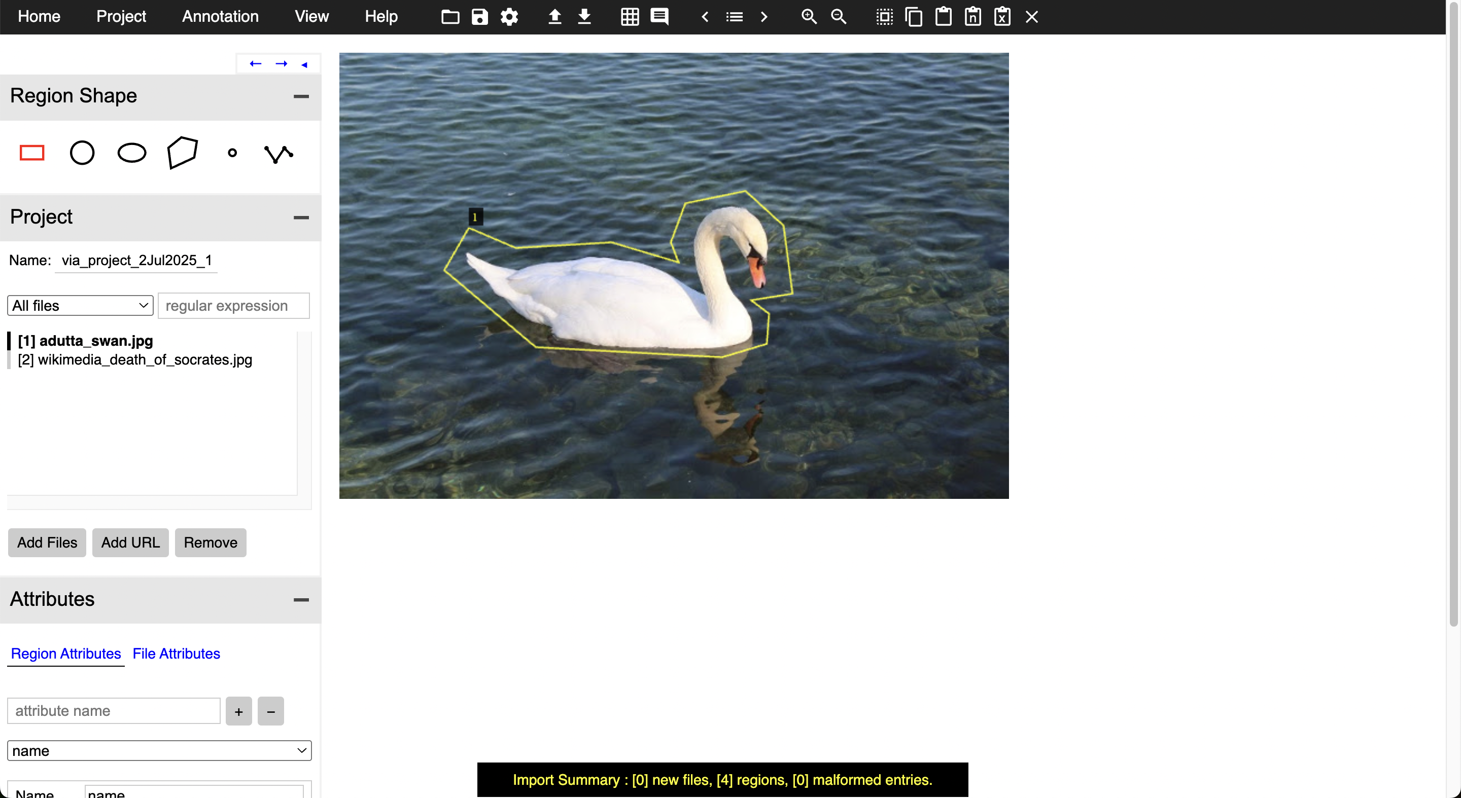
I had to be very familiar with the VGG Image Annotator (VIA) software. It was a little clunky at first, and it was difficult to set the annotation formats at first. One of our team members deployed a VIA server and had the whole flow centralized. If you’re interested in seeing the images, making a public benchmark dataset is still being talked about.
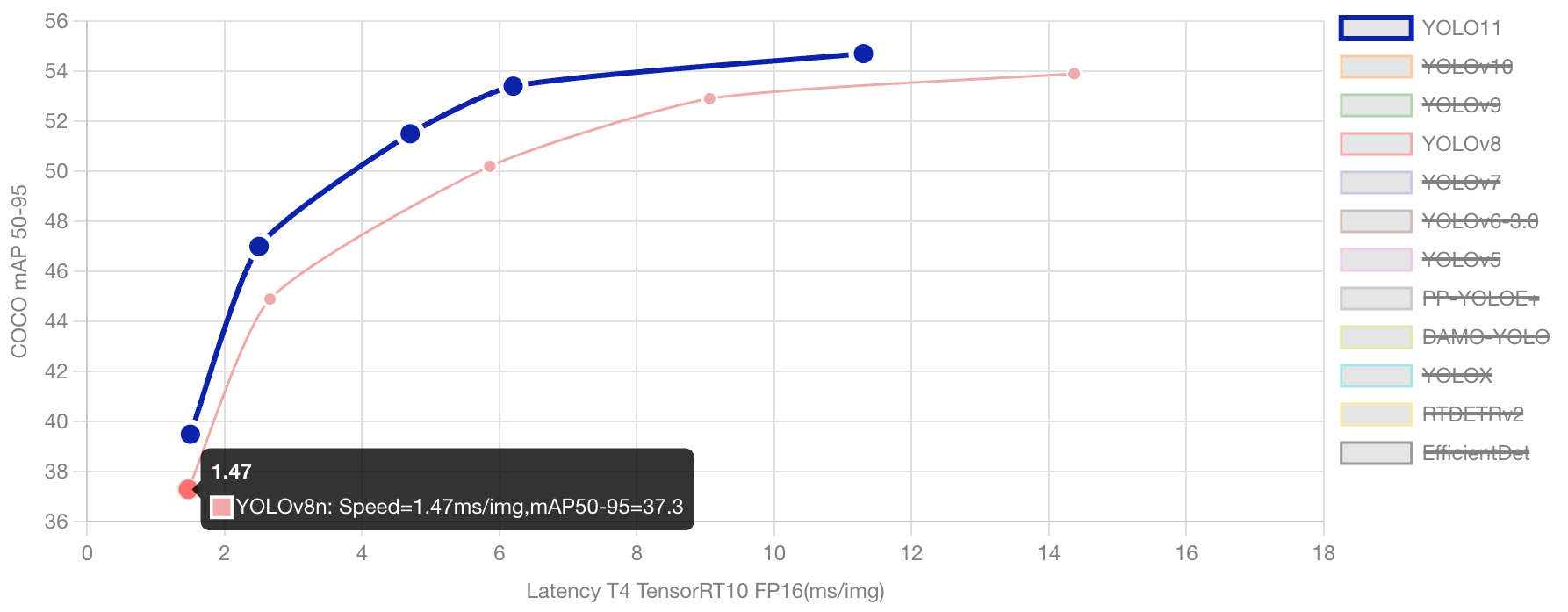
My strategy started off by varying the version and model sizes of the YOLO models I utilized. After some search, I started to compare YOLO8 and YOLO11. YOLO8 is still much sought after, especially in quality control, defect detection, real-time management, and retail inventory management, much due to its stability and mature ecosystem. Slowly though, YOLO11 (which was released recently at this point of writing) has been seen to slowly take over, in terms of speed, computational efficiency, and accuracy. See the chart below for a comparison of the two model versions. See the full technical comparison here: https://docs.ultralytics.com/compare/yolov8-vs-yolo11/#ultralytics-yolo11.
Both model versions also had similar sets of sizes. I tested both the largest (x) and smallest sizes (s) for both YOLO8 and YOLO11, bearing in mind that we had limited resources. Note: We made use of UP’s newest A100 clusters, which offers limited use to the AI department even at this time.
- Nano: yolo8n and yolo11n
- Small: yolo8s and yolo11s
- Medium: yolo8m and yolo11m
- Large: yolo8l and yolo11l
- Extra Large: yolo8x and yolo11x
I also used the initial default YOLO hyperparameters in the first phase before our first deliverable.
| Parameter | Type | Value Range | Default | Description |
|---|---|---|---|---|
| mosaic | float | (0.0, 1.0) | 0.5 | Probability of using mosaic augmentation, which combines 4 images. Especially useful for small object detection |
| hsv_v | float | (0.0, 0.9) | 0.4 | Random value (brightness) augmentation range. Helps model handle different exposure levels |
| hsv_s | float | (0.0, 0.9) | 0.7 | Random saturation augmentation range in HSV space. Simulates different lighting conditions |
| hsv_h | float | (0.0, 0.1) | 0.015 | Random hue augmentation range in HSV color space. Helps model generalize across color variations |
| degrees | float | (0.0, 45.0) | 0.373 | Maximum rotation augmentation in degrees. Helps model become invariant to object orientation |
| translate | float | (0.0, 0.9) | 0.45 | Maximum translation augmentation as fraction of image size. Improves robustness to object position |
| scale | float | (0.0, 0.9) | 0.5 | Random scaling augmentation range. Helps model detect objects at different sizes |
| shear | float | (0.0, 10.0) | 0.3 | Maximum shear augmentation in degrees. Adds perspective-like distortions to training images |
| flipud | float | (0.0, 1.0) | 0.01 | Probability of vertical image flip during training. Useful for overhead/aerial imagery |
| fliplr | float | (0.0, 1.0) | 0.5 | Probability of horizontal image flip. Helps model become invariant to object direction |
Truth be told, I could have varied more on the hyperparameters but will leave this to future work. The full list of tunable hyperparameters can be found on the Ultralytics website.
The best YOLO configuration did pretty well on the dataset, but really struggled in cases of poor lighting and partial occlusions. I think the issue lies in the fact that our validation dataset required more diversity in terms of occlusions, lighting, and other visual factors. This was probably more a reflection in the data collection and annotation rather than YOLO’s ability to generalize.
Part 2
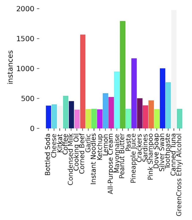
After our first foray, the class was given 2 more weeks to improve the dataset. We added more images, brought up the total number of images per object class to about 500 per grocery item, and double checked our initializations (e.g. ensured the images were of the same sizes, the annotation boxes were correct and in the proper formats, etc.). As you can see here the each class has close to 500 instances each across all images (and a few even went beyond to produce close to 1500!). As this was a coordinated effort, some things were a little out of control individually, but I still think it’s a pretty good start, and it’s nothing a bit of curation can’t help with.
In this phase, I started varying the number of epochs and hyperparameters individually at each experiment. I also introduced some Mixup variations on the dataset during training on Runs 10 and 11. Mixup is a data augmentation technique wherein the training would randomly select pairs of images and linearly interpolate their pixels. You can read more about Mixup from this paper.
I also varied the HSV_v, HSV_s, HSV_h values at the end of this, combining both the increase of epochs (from 30 to 50) and the mixup-affected images. The best model so far was one with the lowest HSV_s in my configuration settings (0.4) with HSV_h and HSV_v kept the same as default (see Part 1).
The tuning would have been better if we had been able to run grid search or Optuna-like mechanisms, or even Ultralytics very own model tuning, this would have been a more correct way to do this. Of course, we were limited by our time-sharing on the A100 NVIDIA units we were assigned to, so I will leave this for future work.
Results
Explanation of the different metrics
| Metric | Values on Best Run | Description |
|---|---|---|
| GPU_mem | 36.1GB | Estimate of memory utilization during training. |
| box_loss | 0.5556 | How well the bounding boxes fit the objects |
| cls_loss | 1.05 | How well the segmentation masks match the objects |
| dfl_loss | 0.9353 | Distribution focal loss, used for better bounding box regression |
| Instances | 3 | Instances seen per image on average |
| P | 0.907 | Precision |
| R | 0.777 | Recall |
| mAP50 | 0.842 | Mean Average Precision at 50% IoU |
| mAP50-95 | 0.734 | More strict average |
Full table of runs
| Run | BoxP | R | mAP | Remarks | |
|---|---|---|---|---|---|
| 1 | 0.910 | 0.800 | 0.879 | Default YOLO-V8 nano, 10 epochs | |
| 2 | 0.946 | 0.901 | 0.922 | Run 1 + Default YOLO-V11 nano | |
| 3 | 0.939 | 0.885 | 0.923 | Run 1 + mosaic=0.5, hsv_h=0.015, hsv_s=0.7, hsv_v=0.4, degrees=0.373, translate=0.45, scale=0.5, shear=0.3, flipud=0.01, fliplr=0.5 | |
| 4 | 0.947 | 0.921 | 0.941 | Run3 with YOLO-V8 medium | |
| 5 | 0.955 | 0.912 | 0.940 | Run3 with YOLO-V11 medium | |
| 6 | 0.951 | 0.919 | 0.940 | Run3 with YOLO-V11 X | |
| 7 | 0.951 | 0.918 | 0.938 | Run6 with CosLR 0.01 to 0.001 | |
| 8 | 0.964 | 0.933 | 0.948 | Run6 with 20 epochs | |
| 9 | 0.964 | 0.958 | 0.974 | Run6 with 30 epochs | |
| 10 | 0.968 | 0.969 | 0.977 | Run9 with Mixup variation on 30 epochs | |
| 11 | 0.969 | 0.977 | 0.974 | Run9 with Mixup variation on 50 epochs | |
| 12 | 0.883 | 0.773 | 0.844 | Made a dataset improvement and reran using Trial 11 settings on 30 epochs | |
| 13 | 0.870 | 0.763 | 0.828 | Trial 12 but on 50 epochs | |
| 14 | 0.898 | 0.785 | 0.842 | Made further dataset improvements and reran using Trial 11 on 30 epochs | |
| 15 | 0.850 | 0.775 | 0.830 | Trial 14 with HSV_h 0.25 | |
| 16 | 0.879 | 0.757 | 0.820 | Trial 14 with HSV_h 0.35 | |
| 17 | 0.845 | 0.775 | 0.817 | Trial 14 with HSV_h 0.45 | |
| 18 | 0.877 | 0.766 | 0.832 | Trial 14 with HSV_s 0.6 | |
| 19 | 0.874 | 0.798 | 0.845 | Trial 14 with HSV_s 0.5 | |
| 20 | 0.907 | 0.777 | 0.842 | Trial 14 with HSV_s 0.4 (Best Run!) | |
| 21 | 0.865 | 0.779 | 0.833 | Trial 14 with HSV_v 0.5 | |
| 22 | 0.846 | 0.785 | 0.839 | Trial 14 with HSV_v 0.6 | |
| 23 | 0.859 | 0.785 | 0.974 | Trial 14 with HSV_v 0.7 |
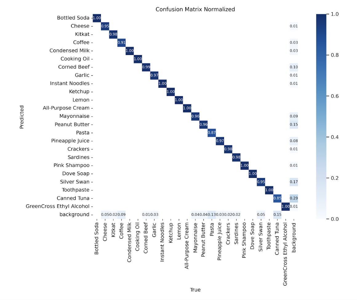
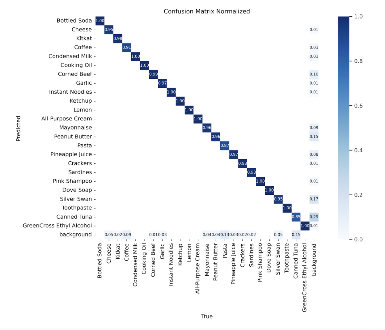
Here is the final confusion matrix from the best configuration’s run.
Training runs
Training runs and weights can be found in this Google Drive. It’s available on a request for access basis.
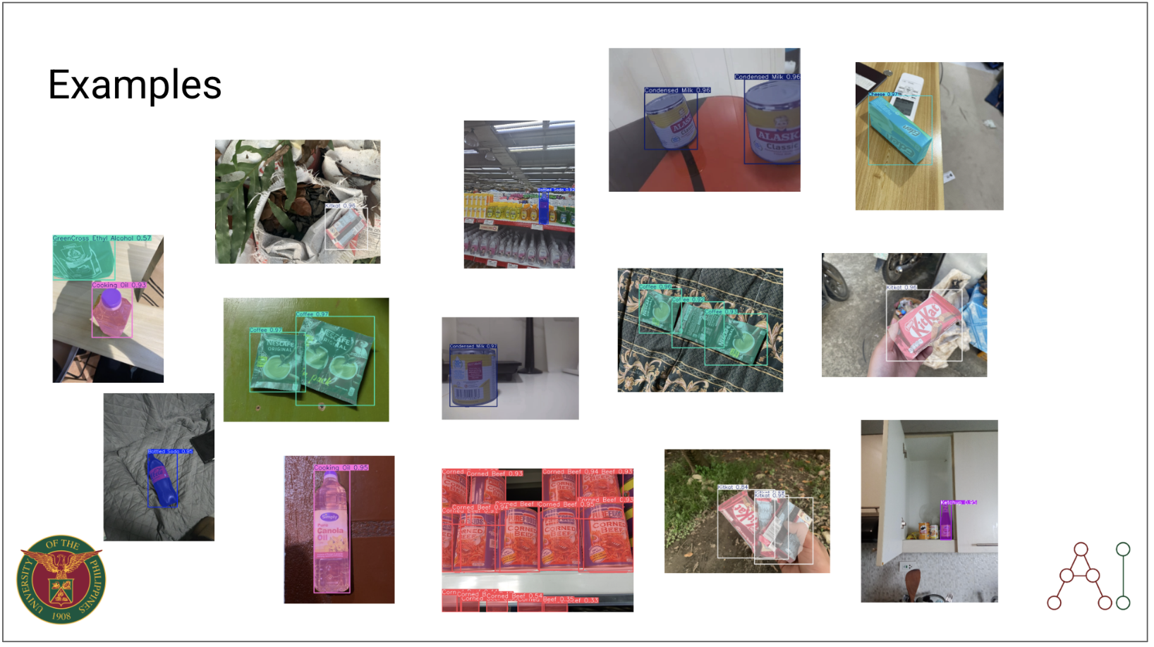
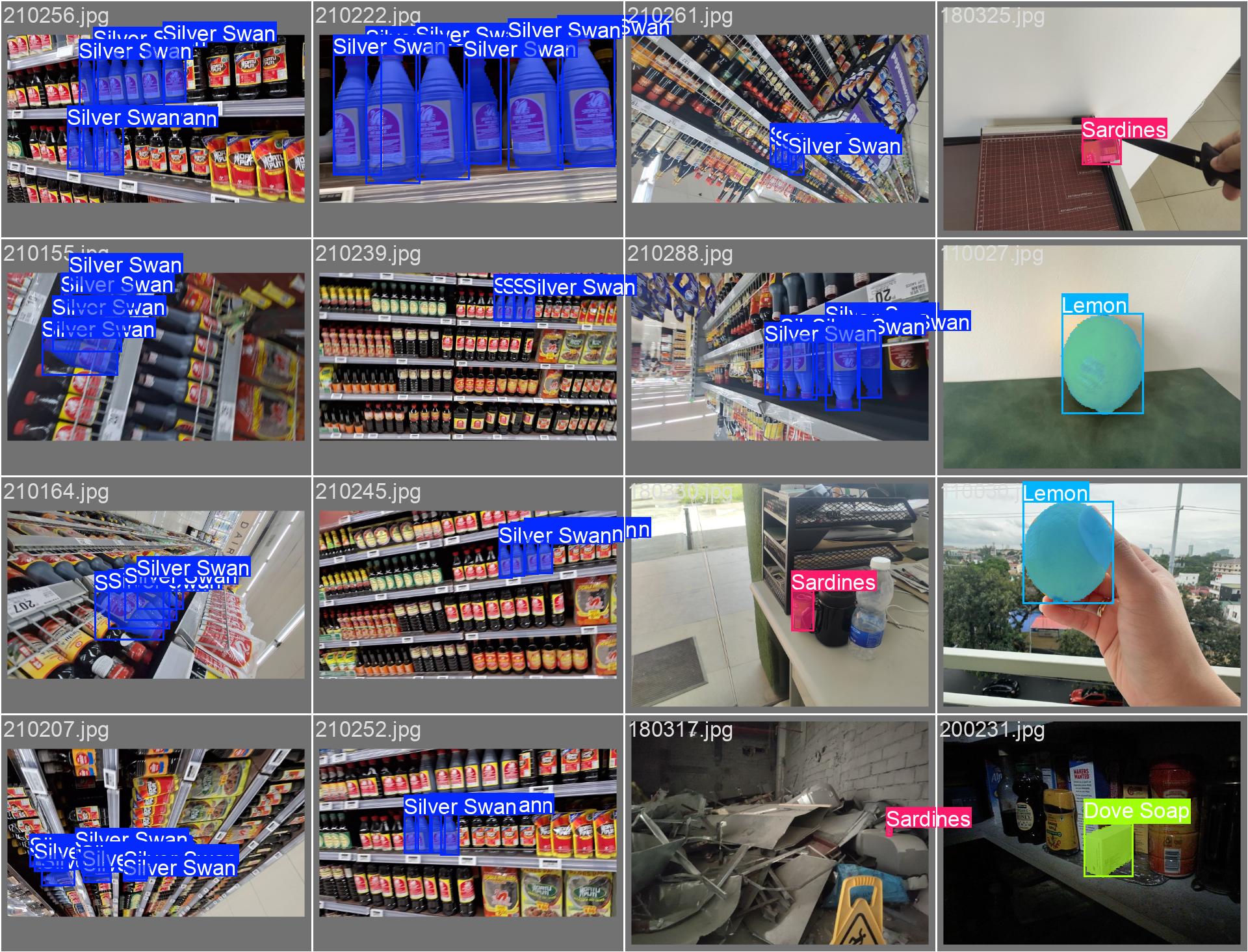
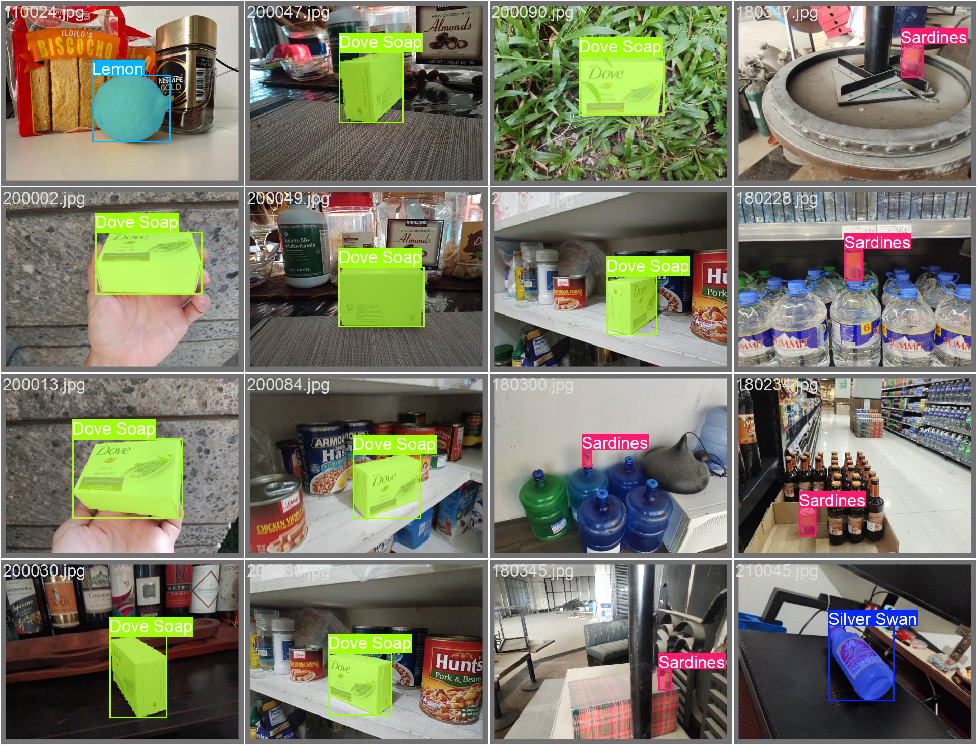
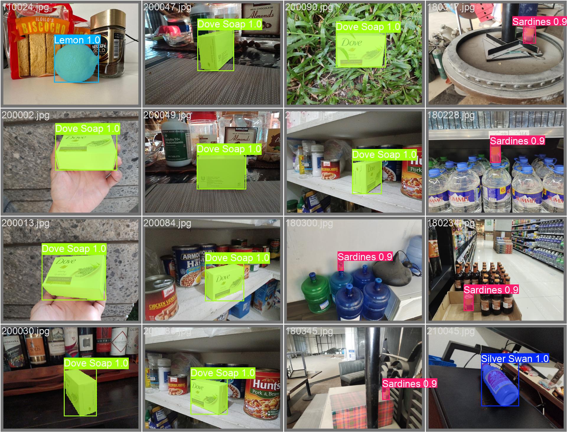
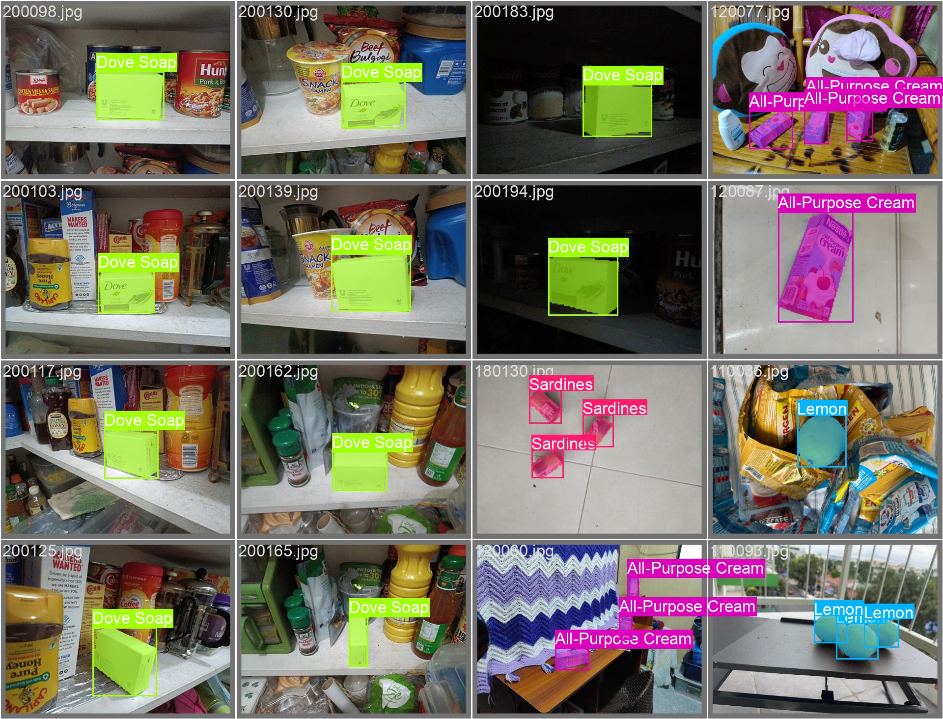
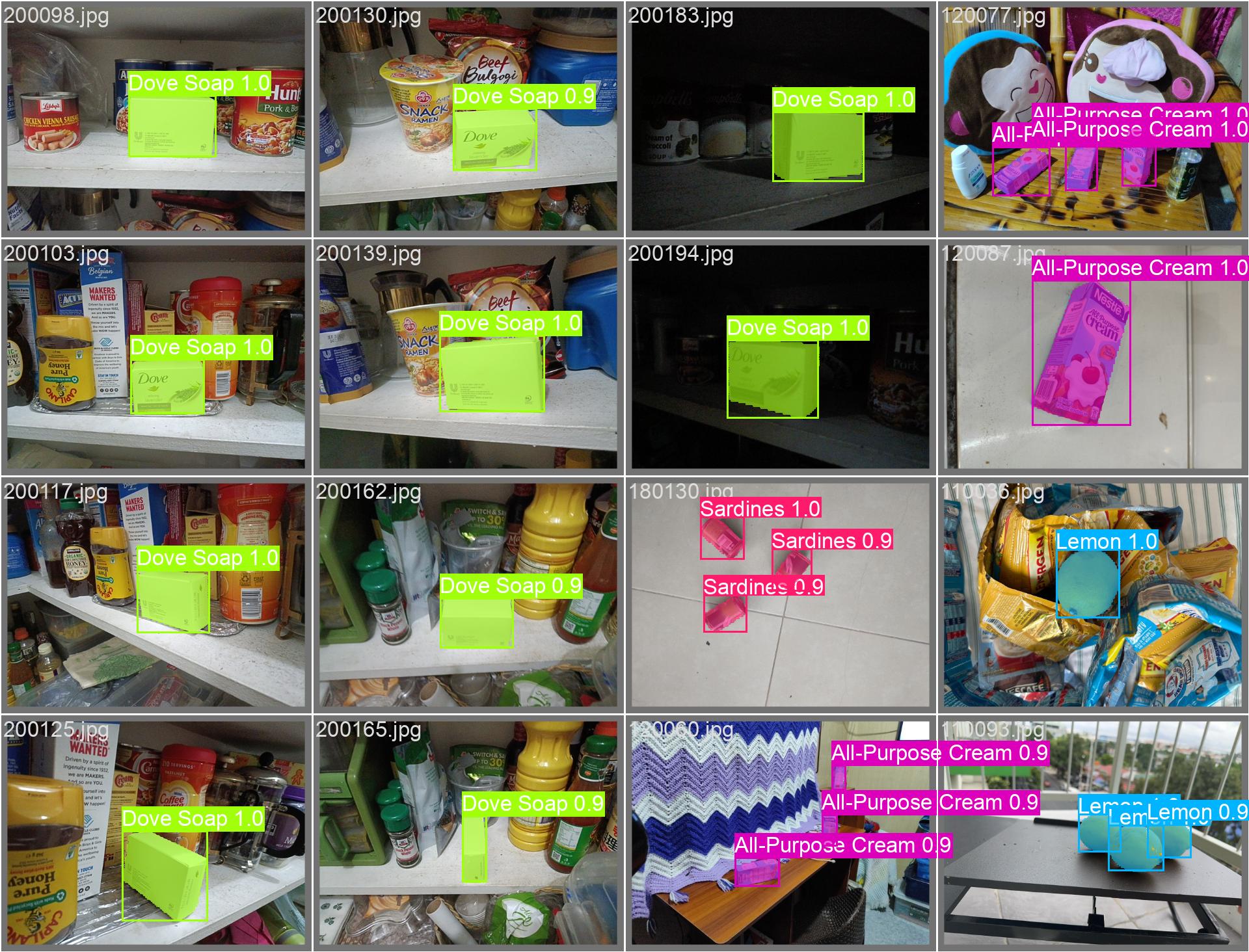
Sample inference
Batch 1: Labelled vs Predicted

Batch 2: Labelled vs Predicted
Batch 3: Labelled vs Predicted
Sample Video
For a sample video, you may look at this Google Drive link.